The n-trailer vehicle
 The n-trailer vehicle has been an exciting topic in three different areas of mathematics; non-holonomic mechanics,
Goursat distribution theory from the point of view of the differential topology, and the monster tower from the point of
view of algebraic geometry. Good references from the point of view of topology: Geometric approach to Goursat flags: Geometric approach to
Goursat flags by Richard Montgomery and Michail Zhitomirskii,
The car with N Trailers
: characterization of the singular configurations by Frédéric Jean .
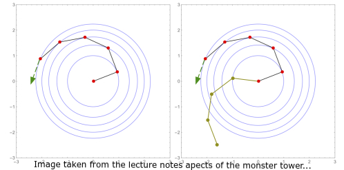
For the approach of algebraic geometry: Points and Curves in the Monster Tower by Richard Montgomery and Michail Zhitomirskii,
Sussan Colley and Gary Kendy see Aspects of the Monster Tower Construction:
Geometric, Combinatorial, Mechanical,Enumerative.
The n-trailer vehicle has been an exciting topic in three different areas of mathematics; non-holonomic mechanics,
Goursat distribution theory from the point of view of the differential topology, and the monster tower from the point of
view of algebraic geometry. Good references from the point of view of topology: Geometric approach to Goursat flags: Geometric approach to
Goursat flags by Richard Montgomery and Michail Zhitomirskii,
The car with N Trailers
: characterization of the singular configurations by Frédéric Jean .
For the approach of algebraic geometry: Points and Curves in the Monster Tower by Richard Montgomery and Michail Zhitomirskii,
Sussan Colley and Gary Kendy see Aspects of the Monster Tower Construction:
Geometric, Combinatorial, Mechanical,Enumerative.
Luis Garcia-Narajo and I studied the dynamics of an articulated n-trailer vehicle that moves under its own inertia, for more details and pictures see The dynamics of an articulated n-trailer vehicle. A. Ardentov and P. Mashtakov made a nilpotent approximation method for the approximate solution for optimal control problem for th n-trailer system in the case n=1, see Control of a Mobile Robot with a Trailer Based on Nilpotent Approximation .
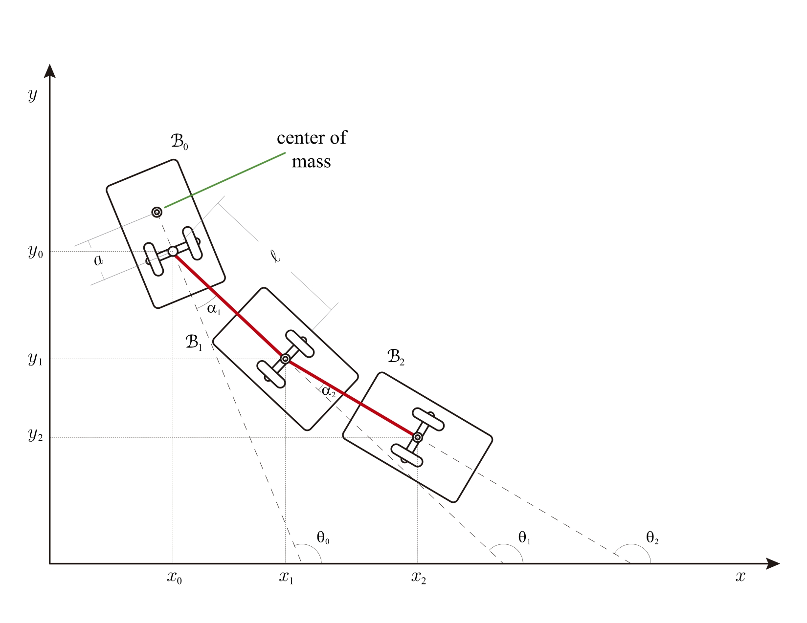
The n-trailer system consists of a leading car (B_0 in the left image), or truck pulling n trailers (B_i with i>1 in the left image), like a luggage carrier in the airport. The wheels on the car and each truck impose a nonholonomic constraint that forbids any motion of the given body in the direction perpendicular to its central axis. The space of configuration Q is SE(2) times T^n ( Euclidean group SE(2) and n-torus T^n), that is, an (n+3)-dimensional manifold, (x_0,y_0,theta_0,theta_1..,theta_n) are the local coordinates for Q following the left picture, here (x_0,y_0) is the contact point of the first car, theta_0 is the angle between the x-axes and car axis (Car B_0). Also, theta_i is the angle between the x-axes and the axis of the trailer B_i where.
 Q is endowed with a Lagrangian function given by the kinetic energy and a two-rank non-integrable distribution D.
SE(2) acts on Q, the lagrangian function, and the distribution D are invariant under the action, the quotient of
Q by SE(2) is an n-torus T^n. The system has two external parameters, namely, "a" and "ell"; the distance between
the center of mass of the leading car (the red point in the left image) and the contact point. We assume that the
center of mass of the trailers B_i is on the contact (x_i,y_i) for all i > 0. ell is the distance of the chain
that joins the car B_k with B_{k-1} (both parameters are defined in the picture). We wrote the equations of motion
on the reduced space (u,omega,T^n), that is, the space of quasi-velocities and T^n. The system is autonomous then
the energy is a constant of motion. The dynamics have a dramatic change when a is zero.
Q is endowed with a Lagrangian function given by the kinetic energy and a two-rank non-integrable distribution D.
SE(2) acts on Q, the lagrangian function, and the distribution D are invariant under the action, the quotient of
Q by SE(2) is an n-torus T^n. The system has two external parameters, namely, "a" and "ell"; the distance between
the center of mass of the leading car (the red point in the left image) and the contact point. We assume that the
center of mass of the trailers B_i is on the contact (x_i,y_i) for all i > 0. ell is the distance of the chain
that joins the car B_k with B_{k-1} (both parameters are defined in the picture). We wrote the equations of motion
on the reduced space (u,omega,T^n), that is, the space of quasi-velocities and T^n. The system is autonomous then
the energy is a constant of motion. The dynamics have a dramatic change when a is zero.
The following videos show the different behaviors of the system. The car's color is green, its center of mass is the red point, and the trailers' color are blue.
Case a different of zero
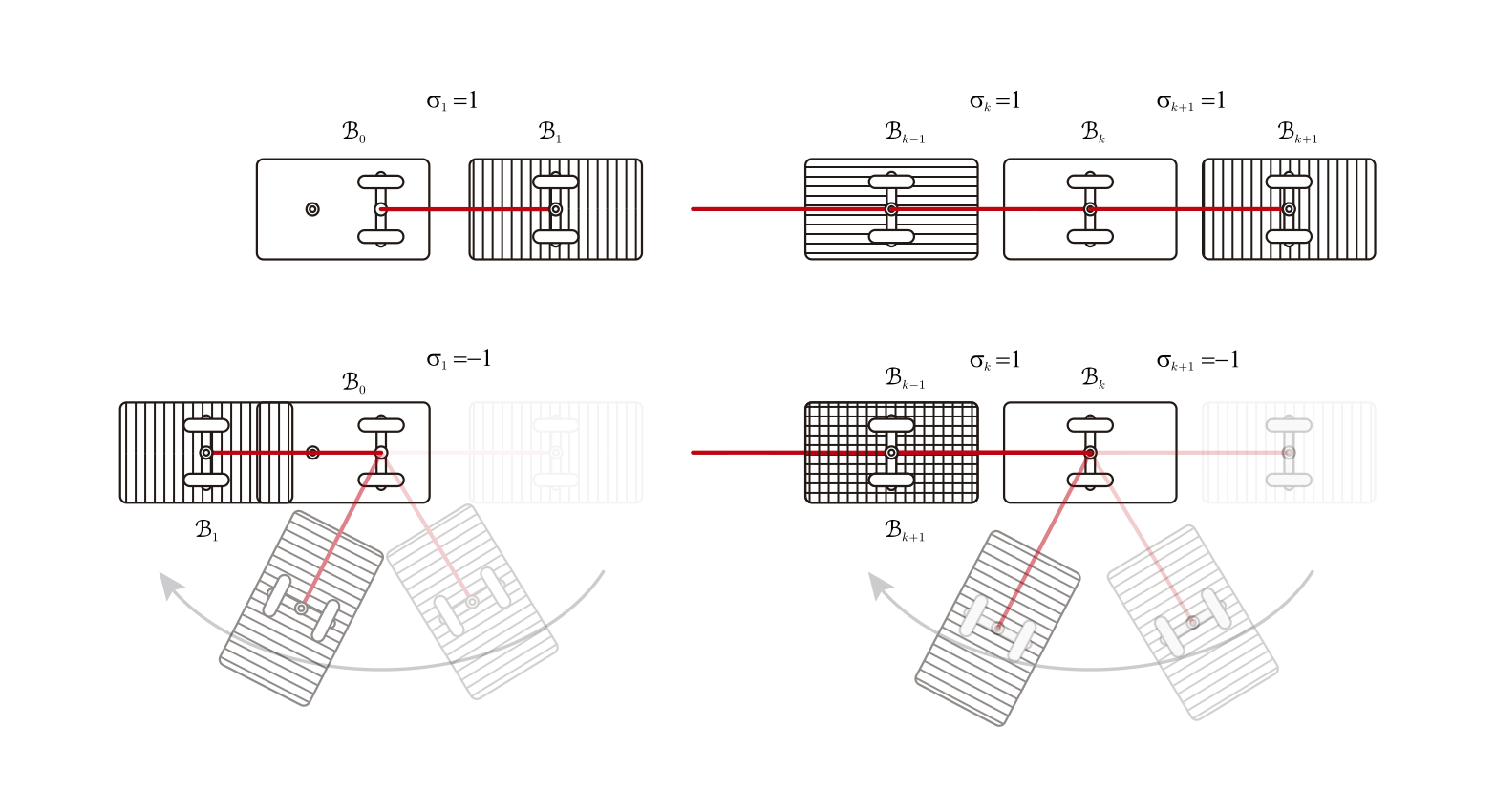
In the case a difference of zero, the energy levels are diffeomorphic to a (n+1)-torus T^{n+1}, the system has 2^n equilibrium points. All of them are hyperbolic (the linear part has all the eigenvalues with real part different of zero. Moreover, the imaginary part is always zero), one is always a sink (all the eigenvalues are negative), other is a source (all the eigenvalues are positive), if they are more, they are saddle points.
The right image shows the configuration of the trailer for different equilibrium points, we used the sigma_k = 1 for the stable position and sigma_k = -1 for unstable position, that is, if sigma_k = 1, then B_k is behind B_{k-1}, if sigma_k = -1 then B_k overlaps with B_{k-1}. The situation resembles the equilibria of a chain of n coupled planar pendula
Case n=1
The following videos show a well-known phenomenon; the stable relative equilibrium points correspond to configurations of the system when the center of mass is located forward in the direction of the movement. In the following videos, the system starts with a small angular velocity, and it reaches its maximum before being asymptotic to 0, smaller maximum angular velocity (Example 1), medium maximum angular velocity (Example 2) and bigger maximum angular velocity (Example 1), medium maximum angular velocity (Example 2) and bigger maximum angular velocity (Example 3). .
Case a=0
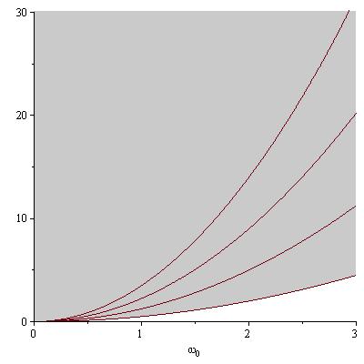 If a = 0, the system has a new constant of motion, namely, the angular velocity of the leading car,
which we call omega. In this case, the energy level is diffeomorphic to T^n. To study the dynamics, we introduce the
space of momentum-Energy parameters (omega,E). The dynamics changes have n critical parabolic curves (see left picture).
They divide the first quadrant (omega > 0 and E >0) in (n+1) disconnected regions. The dynamics corresponding to the
first region do not have equilibrium points. The dynamics of the first critical curve have one invariant manifold of
dimension (n-1); the dimension of the hyperbolic parts is (n-2), and the central manifold has dimension 1.
The second region has two hyperbolic invariant manifolds of dimension (n-1). The second critical curve has two
invariant manifolds of dimension (n-2); the dimension of the hyperbolic parts is (n-3), and the central manifold has
dimension 1. The third region has four hyperbolic invariant manifolds of dimension (n-2), and so on.
If a = 0, the system has a new constant of motion, namely, the angular velocity of the leading car,
which we call omega. In this case, the energy level is diffeomorphic to T^n. To study the dynamics, we introduce the
space of momentum-Energy parameters (omega,E). The dynamics changes have n critical parabolic curves (see left picture).
They divide the first quadrant (omega > 0 and E >0) in (n+1) disconnected regions. The dynamics corresponding to the
first region do not have equilibrium points. The dynamics of the first critical curve have one invariant manifold of
dimension (n-1); the dimension of the hyperbolic parts is (n-2), and the central manifold has dimension 1.
The second region has two hyperbolic invariant manifolds of dimension (n-1). The second critical curve has two
invariant manifolds of dimension (n-2); the dimension of the hyperbolic parts is (n-3), and the central manifold has
dimension 1. The third region has four hyperbolic invariant manifolds of dimension (n-2), and so on.
Case n=1
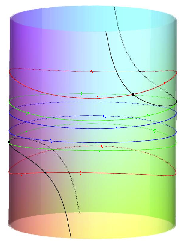 The reduced dynamics is integrable and has a singular energy level E_c (green curve in the cylinder to the right):
Energy E less than E_c (blue curve in the cylinder), the reduce dynamics is periodic and its reconstruction are periodic (Periodic Orbit)
or quasi-periodic (Quasi-periodic Orbit). Energy E equal E_c, the reduced dynamics
is a homoclinic connections whose equilibrium point correspond to periodic solutions in the reconstructed dynamics
( Homoclinic Orbit). Energy E (red curve in the cylinder) is bigger than E_c, the reduced dynamics is a
heteroclinic connection, and its reconstructed dynamics is asymptotic to a periodic solution corresponding to
the equilibrium points (the back curve in the cylinder) (Heteroclinic Orbit).
The reduced dynamics is integrable and has a singular energy level E_c (green curve in the cylinder to the right):
Energy E less than E_c (blue curve in the cylinder), the reduce dynamics is periodic and its reconstruction are periodic (Periodic Orbit)
or quasi-periodic (Quasi-periodic Orbit). Energy E equal E_c, the reduced dynamics
is a homoclinic connections whose equilibrium point correspond to periodic solutions in the reconstructed dynamics
( Homoclinic Orbit). Energy E (red curve in the cylinder) is bigger than E_c, the reduced dynamics is a
heteroclinic connection, and its reconstructed dynamics is asymptotic to a periodic solution corresponding to
the equilibrium points (the back curve in the cylinder) (Heteroclinic Orbit).
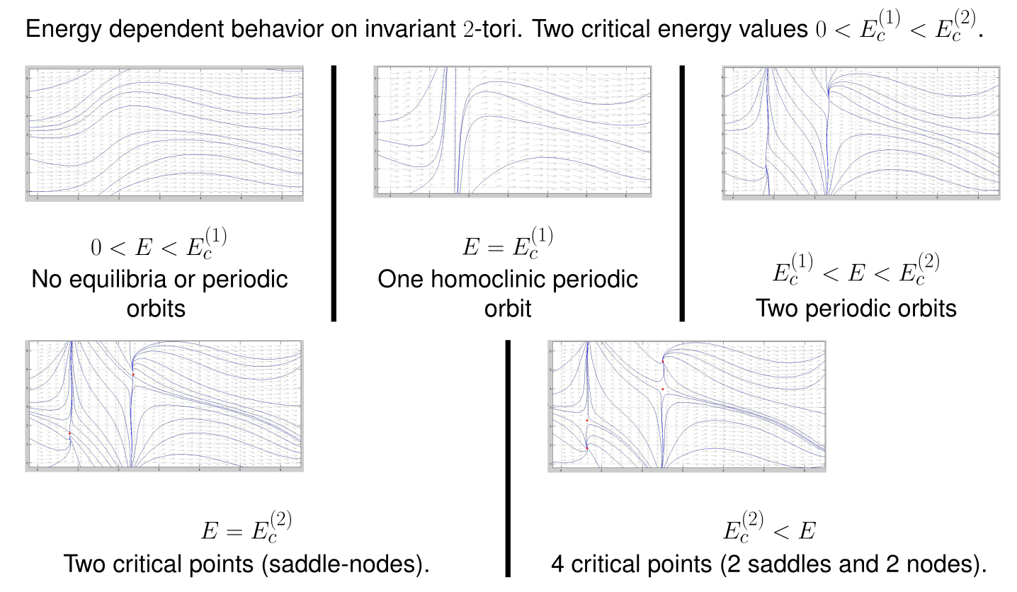
Case n=2
The dynamics have two singular energy levels E1_c < E2_c, see
(Orbit with energy E1_c) and ( Orbit with energy E2_c)
. A solution with energy E < E1_c is (Orbit with E < E1_c
), a solution with energy E1_c < E < E2_c is (E1_c < E < E2_c ) and a solution with energy E2_c < E
< E2_c is (E2_c < E )